Attaching package: 'kableExtra'

The following object is masked from 'package:dplyr':

    group_rows
#Read the penguins_samp1 data file from githubpenguins <-read_csv("https://raw.githubusercontent.com/mcduryea/Intro-to-Bioinformatics/main/data/penguins_samp1.csv")
Rows: 44 Columns: 8
── Column specification ────────────────────────────────────────────────────────
Delimiter: ","
chr (3): species, island, sex
dbl (5): bill_length_mm, bill_depth_mm, flipper_length_mm, body_mass_g, year

ℹ Use `spec()` to retrieve the full column specification for this data.
ℹ Specify the column types or set `show_col_types = FALSE` to quiet this message.
#See the first six rows of the data we've read in to our notebookpenguins %>%head()%>%kable() %>%kable_styling (c("striped", "hover"))
species
island
bill_length_mm
bill_depth_mm
flipper_length_mm
body_mass_g
sex
year
Gentoo
Biscoe
59.6
17.0
230
6050
male
2007
Gentoo
Biscoe
48.6
16.0
230
5800
male
2008
Gentoo
Biscoe
52.1
17.0
230
5550
male
2009
Gentoo
Biscoe
51.5
16.3
230
5500
male
2009
Gentoo
Biscoe
55.1
16.0
230
5850
male
2009
Gentoo
Biscoe
49.8
15.9
229
5950
male
2009
The table represents the penguin species, islands they inhabit, bill length, bill depth, flipper length, and body mass. This data will be used for further analysis.
You can add options to executable code like this.
[1] 4
The echo: false option disables the printing of code (only output is displayed).
About Our Data
The data we are working with is a dataset on penguins, which includes 8 features measured on 44 penguins. The features included are physiological features (like bill length, bill depth, flipper length, body mass, etc) as well as other features like the year that the penguin was observed, the island the penguin was observed on, the sex, and the species of the penguin.
Interesting Questions to Ask
We ask these questions to differentiate among species, sex, and island. Analyzing these differences may suggest evolutionary or adaptive changes developed by the penguins.
What is the average flipper length? What about for each species?
Are there more male or female penguins? What about per island or species?
What is the average body mass? What about by island? By species? By sex?
What is the ratio of bill length to bill depth for a penguin? What is the overall average of this metric? Does it change by species, sex, or island?
Does average body mass change by year?
Data Manipulation Tools and Strategies
We can look at individual columns in a data set or subsets of columns in a dataset. For example, if we are only interested in flipper length and species, we can select() those columns. Here we look at body mass and species to determine if there is an association between species and size. By analyzing this data, we can determine if some species are smaller or larger than others in this dataset.
If we want to filter() and only show certain rows, we can do that too. Here, we use the filter() function to analyze bill length and bill depth by species and island. Analysis of this data may show differences between bill length and bill depth by species or geographical location, which may pose further research questions. What about the environment or evolution of the species causes these differences? However, in this dataset there are not the same amount of penguins per species, which causes difficulty making statements about the species in the dataset. Because we have a large amount of Adelie penguins, we may draw conclusions about that species in this dataset, but with a small amount of Chinstrap and Gentoo penguins, it is difficult to draw conclusions that may speak to the species as a whole.
#we can filter by species (categorical variables) penguins %>%filter(species =="Chinstrap")
# A tibble: 2 × 8
species island bill_length_mm bill_depth_mm flipper_le…¹ body_…² sex year
<chr> <chr> <dbl> <dbl> <dbl> <dbl> <chr> <dbl>
1 Chinstrap Dream 55.8 19.8 207 4000 male 2009
2 Chinstrap Dream 46.6 17.8 193 3800 fema… 2007
# … with abbreviated variable names ¹flipper_length_mm, ²body_mass_g
#we can also filter by numerical variablespenguins %>%filter(body_mass_g >=6000)
# A tibble: 2 × 8
species island bill_length_mm bill_depth_mm flipper_leng…¹ body_…² sex year
<chr> <chr> <dbl> <dbl> <dbl> <dbl> <chr> <dbl>
1 Gentoo Biscoe 59.6 17 230 6050 male 2007
2 Gentoo Biscoe 49.2 15.2 221 6300 male 2007
# … with abbreviated variable names ¹flipper_length_mm, ²body_mass_g
#we can also do bothpenguins %>%filter ((body_mass_g >=6000)|(island =="Torgersen"))
# A tibble: 7 × 8
species island bill_length_mm bill_depth_mm flipper_l…¹ body_…² sex year
<chr> <chr> <dbl> <dbl> <dbl> <dbl> <chr> <dbl>
1 Gentoo Biscoe 59.6 17 230 6050 male 2007
2 Gentoo Biscoe 49.2 15.2 221 6300 male 2007
3 Adelie Torgersen 40.6 19 199 4000 male 2009
4 Adelie Torgersen 38.8 17.6 191 3275 fema… 2009
5 Adelie Torgersen 41.1 18.6 189 3325 male 2009
6 Adelie Torgersen 38.6 17 188 2900 fema… 2009
7 Adelie Torgersen 36.2 17.2 187 3150 fema… 2009
# … with abbreviated variable names ¹flipper_length_mm, ²body_mass_g
Answering Our Questions
Most of our questions involve summarizing data, and perhaps summarizing over groups. We can summarize data using the summarize() function and group data using group_by().
Let’s find the average flipper length. Table 1 shows the overall flipper length average, while Table 2 shows the average flipper length in the Gentoo species, and Table 3 represents average flipper length across the 3 species individually. This data shows that the Gentoo penguins had the largest average flipper length. These tables were created using the summarize() and group_by() functions.
#Overall average flipper lengthpenguins %>%summarize(avg_flipper_length =mean(flipper_length_mm))
# A tibble: 1 × 1
  avg_flipper_length
               <dbl>
1               212.
#Single Species Averagepenguins %>%filter(species =="Gentoo") %>%summarize(avg_flipper_length =mean(flipper_length_mm))
# A tibble: 3 × 2
  species   avg_flipper_length
  <chr>                  <dbl>
1 Adelie                  189.
2 Chinstrap               200
3 Gentoo                  218.
How many of each species do we have? This can be found using the count() function. This is important when analyzing and comparing quantitative data to ensure accuracy, especially when drawing conclusions in a dataset.
penguins %>%count(species)
# A tibble: 3 × 2
  species       n
  <chr>     <int>
1 Adelie        9
2 Chinstrap     2
3 Gentoo       33
How many of each sex are there? What about by island or species? When measuring anatomic features of animals, sex is important, as in some species, certain traits are particular to one sex of the species.
penguins %>%count(sex)
# A tibble: 2 × 2
  sex        n
  <chr>  <int>
1 female    20
2 male      24
penguins%>%group_by(species) %>%count(sex)
# A tibble: 6 × 3
# Groups:   species [3]
  species   sex        n
  <chr>     <chr>  <int>
1 Adelie    female     6
2 Adelie    male       3
3 Chinstrap female     1
4 Chinstrap male       1
5 Gentoo    female    13
6 Gentoo    male      20
We can use mutate() to add new columns to our data set. Here we found the average bill length to depth ratio, first in the dataset as a whole, and then by species, using the mutate(), summarize(), and group_by() functions. The data suggests that the Gentoo penguins have the largest bill length to depth ratio, but it must again be remembered that there is a much larger sample of Gentoo penguins compared to the other species. Additionally, there is a large amount of male penguins in the species, which in many species are found to be the larger of the sex, and therefor develop larger features, potentially like bills. To gather a better understanding regarding differences among species, the dataset would require more even amounts of penguins per species.
#To make a permanet change, we need to store the results of our manipulationspenguins_with_ratio <- penguins %>%mutate(bill_ltd_ratio = bill_length_mm /bill_depth_mm)#Average Ratio penguins %>%mutate(bill_ltd_ratio = bill_length_mm /bill_depth_mm) %>%summarize (mean_bill_ltd_ratio =mean(bill_ltd_ratio),median_bill_ltd_ratio =median(bill_ltd_ratio))
Here we find average body mass by year. In animal species, body mass can fluctuate by year. Fluctuations where average body mass by year drops drastically or declines slowly may be cause for concern, and can be caused by loss of environment, lack of food, disease, competition, etc. The steady decline in average body mass from 2007-2009 represented by the table may be worrisome for the penguin populations in this dataset.
# A tibble: 3 × 2
   year mean_body_mass
  <dbl>          <dbl>
1  2007          5079.
2  2008          4929.
3  2009          4518.
Data Visualization
What is the distribution of penguin flipper lengths?
What is the distribution of penguin species?
Does the distribution of flipper length depend on the species of penguin?
Is there a correlation between bill length and bill depth?
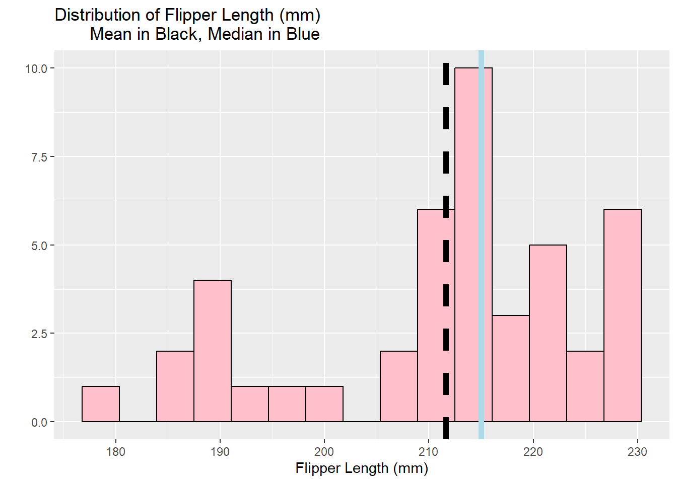
penguins %>%ggplot () +geom_histogram( aes(x = flipper_length_mm), bins =15, fill ="pink" , color ="black")+labs(title ="Distribution of Flipper Length (mm) Mean in Black, Median in Blue", y ="", x ="Flipper Length (mm)") +geom_vline (aes(xintercept =mean(flipper_length_mm)) , lwd =2, lty ="dashed") +geom_vline (aes(xintercept =median (flipper_length_mm)), color ="lightblue" , lwd =2, lty ="solid")
Warning: Using `size` aesthetic for lines was deprecated in ggplot2 3.4.0.
ℹ Please use `linewidth` instead.
Above, we created a histogram to visualize the distribution of penguin flipper lengths. The black dashed line represents the dataset mean, and the blue solid line represents the dataset median. In this dataset, the average flipper length appears to range from about 205-215 mm, the lowest flipper length is around 170 mm, and the highest flipper length is 230 mm. This graph shows us how flipper length ranges across the dataset, but without species, island, or sex specification, it becomes difficult to differentiate the data for analysis.
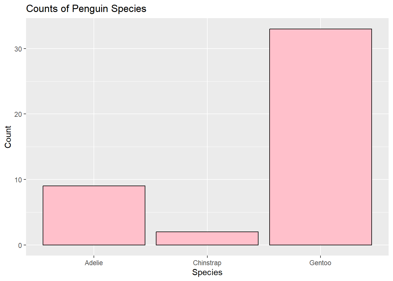
We will now look at the distribution of species, using a histogram. This graph shows us that there is a significantly larger amount of Gentoo penguins than Adelie and Chinstrap. These numbers may skew analysis when grouping and comparing by species.
penguins %>%ggplot() +geom_bar(mapping =aes(x = species), fill ="pink", color="black") +labs(title ="Counts of Penguin Species" , x ="Species", y ="Count")
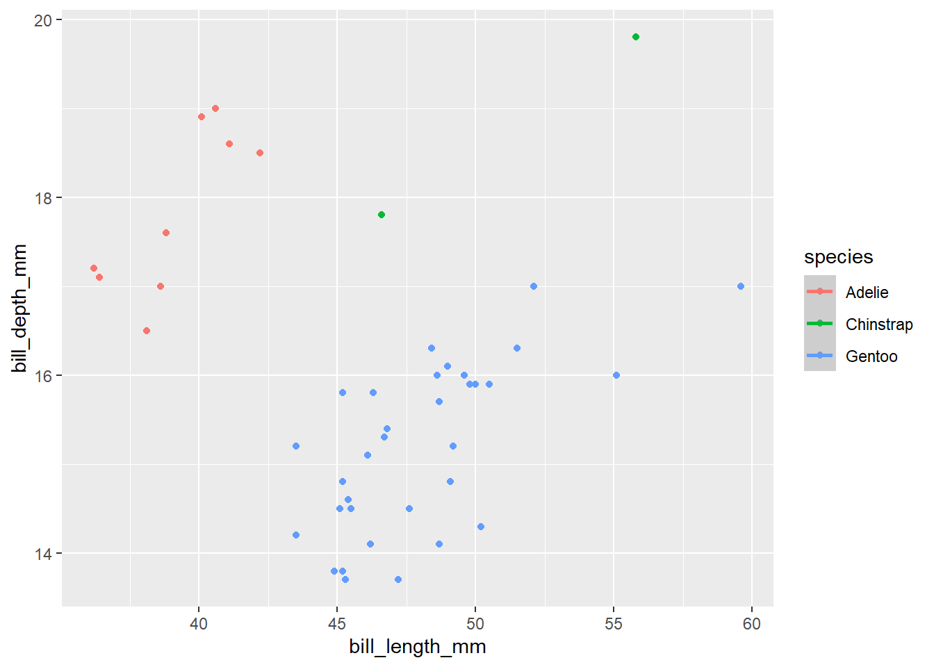
Let’s make a scatter plot to determine if bill length is correlated with bill depth. The scatter plot shows that bill length is not necessarily correlated with bill depth, and different species show different associations between the two. The Adelie penguins showed significantly higher bill depth than the Gentoo species, but the Gentoo species showed significantly higher bill length than the Adelie penguins. The Chinstrap penguins show relatively high bill lengths and bill depths, but this is a difficult comparison to make because there are only 2 Chinstrap penguins, compared to the much larger populations of Gentoo and Adelie penguins in this dataset.
penguins %>%ggplot() +geom_point(aes (x= bill_length_mm, y= bill_depth_mm, color = species))+geom_smooth(aes (x= bill_length_mm, y=bill_depth_mm, color = species))
`geom_smooth()` using method = 'loess' and formula = 'y ~ x'
Warning in simpleLoess(y, x, w, span, degree = degree, parametric =
parametric, : span too small. fewer data values than degrees of freedom.
Warning in simpleLoess(y, x, w, span, degree = degree, parametric =
parametric, : at 46.554